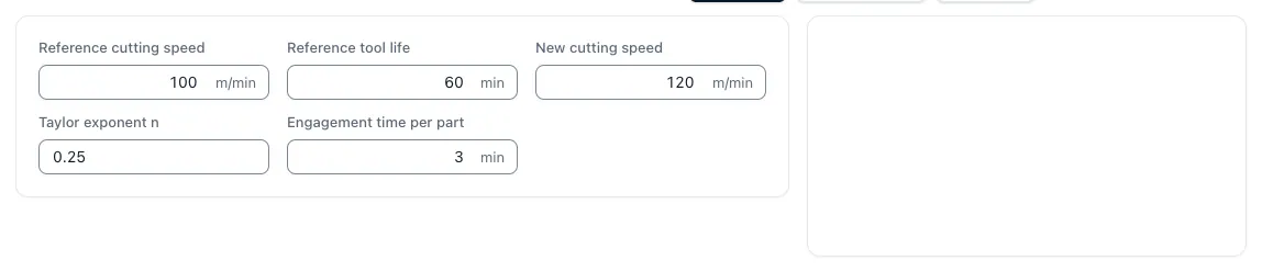
The service life follows the Taylor straight vc × T^m = constant: The service life for a different cutting speed can be calculated from a known value pair. Due to the intervention time per part, it results in the stand quantity and thus the tool costs per component.
Formulas
vc × T^m = konstantTaylor Straight
The classic connection between cutting speed and service life.
T = T₀ × (vc₀ ÷ vc)^(1/m)Switched to service life
A known value pair becomes the service life for a new speed.
Teile je Schneide = T ÷ t_EingriffLevel
The service life divided by the operating time per component.
k_WZ = (Werkzeugkosten + Wechselkosten) ÷ StandmengeTool costs per component
Only with this will the selection of cutting data be economically comparable.
Example: increase vc from 150 to 180 m/min
Reference: 45 minutes service life at 150 m/min, coated carbide (m = 0.25), 2.5 minutes service life per component, 18 € tool costs per service life, 4 minutes change time at 72 €/h.
- Running time at 180 m/min = 45 × (150 ÷ 180)⁴21.7 min
- Life loss−51,8 %
- Components per cutting edge before = 45 - 2,518 pc.
- Time of intervention afterwards = 2,5 × 150 ÷ 1802,08 min
- Components per cutting edge afterwards = 21.7 ÷ 2.0810,4 pc.
- Cost Tool change = 4 ÷ 60 × 724,80 €
- Tool costs per component afterwards = 22,80 ÷ 10,42,19 €
ResultThe tool costs per component rise from 1.27 € to 2.19 € – the intervention time, on the other hand, decreases by only around 17 percent.
At 72 €/h, the higher speed saves 0.50 € machine time per part, but costs 0.92 € more tool. In this case, the faster setting is more expensive.
Service life, service life and level
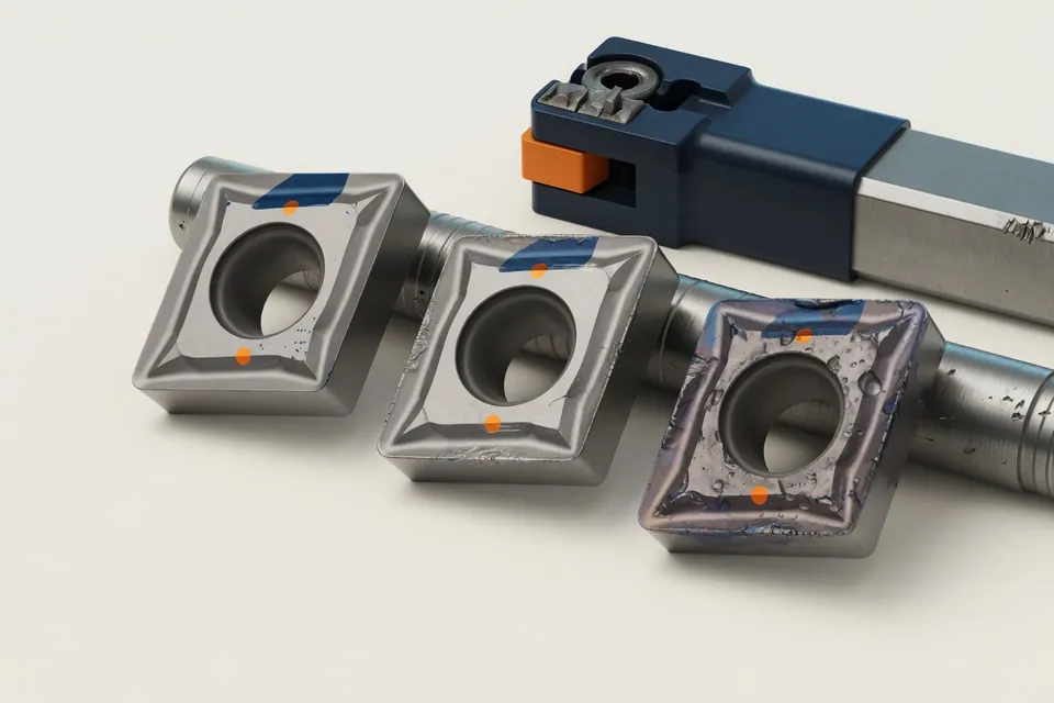
The service life T is the time in operation that a cutting edge works until a specified service life criterion is reached. Wear marks such as the width of the wear mark on the open surface (VB) or the colk depth on the chip surface (KT) are common; in operation, dimensional stability, surface or ridge formation often also count.
- Life T: intervention time in minutes to criterion
- Standby path L: progressed during this time, L = T × vf
- Level N: Number of components per cutting edge, N = T ÷ Operating time per part
The operator shall determine which criterion applies and the service life of different sources shall be comparable only if the criterion, material and cutting conditions are identical.
Calculate service life during milling
When milling, only the time in which the tool actually cuts, not rapid movement, positioning or tool change counts. The standing amount is the service life divided by the main time per part, the service life the service life times feed speed.
With the example of this page, 45 minutes of service life at 150 m/min and 2.5 minutes of operation time per component, a cutting edge for 18 components is sufficient. At an assumed feed speed of 800 mm/min, it travels 36.0 m of service life. At 180 m/min and the same tooth feed, the feed speed increases to 960 mm/min, but the service life drops to 21.7 minutes: the service life shrinks to 20.8 m.
N = T ÷ t_h · L = T × vf
How the tool costs per component, including change time and regrinding, become out of the stand quantity, shows Making tool costs per part; the app calculates it in the tool "Tool costs per part" .
Service life and cost per part above the cutting speed
As the cutting speed increases, the operating time per part decreases only in a ratio of 150 vc, but the service life according to Taylor with the fourth potency. The table calculates the example of this page for six cutting speeds. Under these assumptions, the sum of tool and machine time costs is the smallest at 135 m/min: 4.26 € per part.
Service life, stand quantity and costs depending on the cutting speed
Example of calculation of this page: 45 minutes service life at 150 m/min, m = 0.25, 2.5 minutes service life at 150 m/min, 18 € tool costs per service life, 4 minutes change time and 72 €/h.
| vc in m/min | Life T | Time of intervention per part | Parts per cutting edge | Tool costs per part | Machine time per part | Total per part |
|---|---|---|---|---|---|---|
| 120 | 109.9 min | 3.13 min | 35,2 | 0,65 € | 3,75 € | 4,40 € |
| 135 | 68,6 min | 2,78 min | 24,7 | 0,92 € | 3,33 € | 4,26 € |
| 150 | 45,0 min | 2,50 min | 18,0 | 1,27 € | 3,00 € | 4,27 € |
| 165 | 30.7 min | 2,27 min | 13,5 | 1,69 € | 2,73 € | 4,41 € |
| 180 | 21.7 min | 2,08 min | 10,4 | 2,19 € | 2,50 € | 4,69 € |
| 200 | 14.2 min | 1.88 min | 7,6 | 3,00 € | 2,25 € | 5,25 € |
The procedure time decreases with the cutting speed because the same way is driven faster with the same tooth feed. Values apply only to these assumptions; the own Taylor exponent and the own reference life move the minimum.
From service life to calculation
Cutting speed and service life are related to the Taylor equation; the formula and guide values of the cutting speed are below Calculate cutting speed. Tool costs and changing times enter the unit costs.
The Fully automatic calculation from drawing and CAD (Pro) combines the times and costs of a part of drawing and CAD model into a calculation design; each value remains comprehensible and you release the design.
The fastest setting is rarely the cheapest
The fastest attitude is rarely the cheapest: Only when machine time, tool costs and change times are evaluated together, the economic attitude is shown.
Questions and answers
What is the service life?
The service life is the time a cutting edge works in the operation until a defined criterion has been reached, for example a certain wear mark width on the free surface, a dimensional deviation or a worse surface. Easiness, positioning and tool changes are not included.
What is the difference between service life, standway and stand quantity?
The service life measures the operating time in minutes, the service life of the feed path (L = T × vf) driven during this time and the service life the number of components per cutting edge (N = T ÷ service life per part). For the calculation, the service life is most useful because it leads directly to the tool costs per part.
How do you calculate the service life during milling?
Only the time during which the cutter cuts is counted. The stand amount follows from the service life and the main time per part: with 45 minutes service life and 2.5 minutes operation per part, one cutting edge is sufficient for 18 parts. For a different cutting speed, the service life is converted to the Taylor equation.
How do you calculate the service life of a tool?
Use the Taylor equation vc × T^m = constant. From a known pair, such as 45 minutes of tool life at 150 m/min, estimate tool life at another cutting speed: T = T₀ × (vc₀ ÷ vc)^(1/m). The exponent m depends on the cutting tool material.
Which Taylor exponent do you take?
The reference values are m ᐅ 0.125 for HSS, 0.25 for coated carbide, 0.35 for cermet and fine grain carbide, and 0.45 for cutting ceramics. The larger m, the less the service life reacts to a change in cutting speed.
Why does more speed cost so much service life?
Because the connection is exponential. At m = 0.25, an increase in cutting speed by 20 percent halves the service life to about half. This is the reason why the fastest setting is rarely the most economical.
When is a higher cutting speed worth it anyway?
If the machine time saved is worth more than the additional tool and change costs. This is exactly what the tool calculates for the service life of the app: Tool costs per component and number of tool changes per 100 parts can be directly held against the machine hourly rate.
Where does the reference value come from?
Best from your own operation: service life protocol, tool management or documented experience on a reference part. Manufacturer specifications are a good starting point, but apply to defined conditions for intervention, cooling and stability.