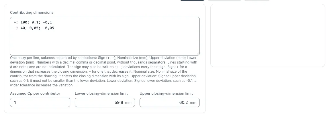
Set the direction of measurement and dimensions
Each dimension is entered with sign, nominal dimension as well as upper and lower dimension. A positive link extends the closing dimension, a negative one shortens it. Therefore, the unfavourable boundary cases are also exchanged accordingly with a deducted dimension.
The calculator processes linear chains. Angular dependencies, spatial geometry, reference systems, elastic deformation or assembly conditions are not automatically modeled.
Example with two dimensions
From 100 ± 0.10 mm less 40 ± 0.05 mm the nominal closing dimension is 60 mm. The smallest value is 99,90 − 40.05 = 59.85 mm; the largest is 100.10 − 39,95 = 60.15 mm.
The worst-case width is thus 0.30 mm. At specified limits of 59.80 and 60.20 mm, these purely geometric border cases are within the permitted range. This presupposes that all relevant dimensions and conditions have been recorded.
Statistical dispersion under fixed assumptions
The computer derives a standard deviation from the tolerance width of each link and the assumed Cp. For independent contributions, the variances are added. For Cp = 1 for both sample dimensions, an RSS standard deviation of around 0.037268 mm results.
Three times this value is about 0.111803 mm. This is not a guaranteed limit range. The model calculation requires independent, central normal distributions and the entered Cp; correlations or process shifts can change this statement.
σ_i = T_i ÷ (6 × Cp); σ_Chain = √Σσ_i²
Example with four dimensions in both directions
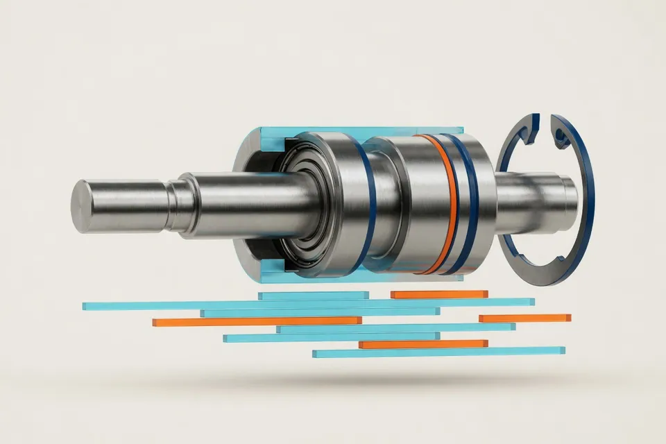
A housing hole of 100 ± 0.10 mm absorbs three parts in a row: a socket 40 ± 0.05 mm, a distance sleeve 25 ± 0.05 mm and a ring 30 ± 0.02 mm. The axial residual gap is sought. The housing dimension counts positively, the three built-in parts count negatively; the nominal closing dimension is 100 − 40 − 25 − 30 = 5 mm.
In the worst case, all dimensions are added: The smallest gap is 99.90 − 40.05 − 25.05 − 30.02 = 4.78 mm, the largest 100.10 − 39.95 − 24.95 − 29.98 = 5.22 mm, i.e. 5 ± 0.22 mm. With the default Cp = 1 of the app, the statistical calculation results in an RSS standard deviation of around 0.041366 mm; three times this value is about 0.124097 mm, i.e. approximately 5 ± 0.124 mm. The statistical width is significantly smaller for four limbs than the worst-case width, but is only valid under the aforementioned distribution assumptions.
Tolerance chain with four dimensions
| Measure | Direction | Nominal dimension | Dimensions | Tolerance T | σ at Cp = 1 |
|---|---|---|---|---|---|
| Housing bore | + | 100 mm | ±0,10 mm | 0,20 mm | 0,033333 mm |
| Box | − | 40 mm | ±0.05 mm | 0,10 mm | 0,016667 mm |
| Distance sleeve | − | 25 mm | ±0.05 mm | 0,10 mm | 0,016667 mm |
| Ring | − | 30 mm | ±0.02 mm | 0,04 mm | 0,006667 mm |
| Locking dimension (column) | 5 mm | Worst case ±0.22 mm | 0,44 mm | RSS 0.041366 mm |
σ_i = T_i ÷ (6 × Cp); σ_stack = √Σσ_i². Use the dimensions from this example in the tolerance stack calculator to reproduce the result.
Statistics does not replace the release of the dimensional chain
The normal model output in the computer outside the limits is a modeled frequency. It is neither a measured part of the reject nor a proof of the assembly capability. If the distribution assumptions or process capabilities are unknown, this estimate remains unsecured.
Check direction, reference conditions and any valid dimensional line. Warnings about omitted invalid lines mean that the result no longer represents the fully intended chain.
Sources and classification
- NIST: Combining uncertainty components
Quadratic combination of independent standard contributions; additional terms are required for correlation.
- NIST: Process Capability
Definition of the ability index Cp. The linear boundary calculation is its own prescriptive interval arithmetic.
Questions and answers
What is a tolerance chain analysis?
A tolerance chain analysis determines how the tolerances of several successive dimensions affect a closing dimension, for example on a game or a distance in a assembly. To this end, the dimensional elements are recorded with direction and dimensions and aggregated to the nominal dimension, maximum and minimum dimensions of the closing dimension.
When do you calculate Worst Case and when statistically?
Worst Case adds all tolerances and guarantees the closing measure for each individual part; this is common with few dimensional elements, individual parts and safety-relevant dimensions. Statistical calculation of the root from the square sum requires independent, centered and stablely manufactured dimensions and allows a small part outside the limit; it is worthwhile with many dimensional elements and series.
Can I simply use statistical tolerances instead of worst case?
Only if the statistical requirements and the permissible risk are technically justified. Worst Case describes permissible boundary combinations; statistics describes an assumed distribution model.
What happens with unbalanced measurements?
The limit calculation uses the upper and lower dimensions with their actual position. The statistical mean is based on the tolerance centers in the model and can therefore differ from the nominal closing dimensions.